It ‘s been 2 weeks since I arrived in Hong Kong. I still cannot get used to the lifestyle here. Everything seems to be strange to me. Here I experience for the first time simultaneously loneliness, pressure, boredom, etc. Today is boring Sunday again. As usual, I get up and go to the library. I think it ‘s the best place that I can come to at the moment. Recently, I have tried to read a well-known Hamilton’s paper that my advisor provided me. It ‘s really difficult paper for those who have just started to study Riemannian Geometry like me. I cannot virtually get anything from the paper these days. Fortunately, during the time I have struggled to understand the paper, I found a great trick that may help us reduce considerably our computation in terms of “tensorial” quantities. Walk on the campus and think about the paper, I thought it ‘s better to note something on my blog.
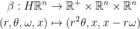
First of all, I would like to mention the motivation of this post. Suppose  is a Riemannian manifold, we concern about several geometric flows that derive from evolution equations like

where  ‘s is a family of Riemannian metric and
  ‘s is a family of some symmetric to tensor. In local coordinate, we may write equations as
  where
where  and
and 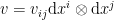 . In several cases, we may be interested in finding the rate of change of Christoffel symbols
  ‘s.
‘s.
To understand this post, readers need to have some basic background on Riemannian Geometry. First of all, I would like to introduce a notion called geodesic normal coordinates. The following result states its existence.
Proposition Let  be a Riemannian manifold. Then at every
  , there exists a local coordinate
  at p such that all of the following hold:
1.  for any
  at the point
  ;
;
2.  for any
  at ;
at ;
3.  for any at
This local coordinate is called the geodesic normal coordinate
Now return to the main problem. We fix a point and a time  . Choose the normal coordinate
  at respect to the metric
  .Recall that Christoffel symbols given by Levi-Civita connection as
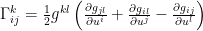
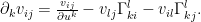
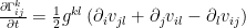
differentiating to both sides, we have
 .
.
That is where the amazing thing comes out. At the point with the normal coordinate, we can simplify our expression above by the fact that the term 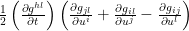 vanishes.
Therefore,
 .
.
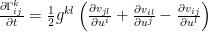
Also, In the normal coordinate, due to the fact that Christoffel symbols vanish, the partial derivative will turn into the covariant derivative by
Finally, we get
 at .
at .
Now, we can see that the LHS is a (1,2)-tensor because the difference of Levi-Civita connections is actually a tensor ( readers can easily check it out by using the definition of Levi-Civita connection). Meanwhile, the RHS is also a tensor of the same kind as it is the contraction of other tensors. To sum up, the RHS and LHS now are independent of the choice of coordinate charts. Because the point vary arbitrarily, we eventually obtain that
for everywhere.
Similarly, we can also establish variations of more complicated quantities such as (1,3)-, (0,4)-Riemmanian tensors, etc.
If we take  , we get celebrated Ricci flow, that was proposed by Hamilton and then used by Perelman to solve famous Poincare conjecture. Such kinds of equalities are really important for analyzing the evolution of curvatures and by that way, Poincare conjecture was solved.