Seriously, why can I come up with a silly question like this? It is probably your first thought when seeing this weird title. But be patient, it is not a joke and I am really serious because I want to convince you that geodesics are actually what they should be.
As we may have heard about geodesics, they are locally minimizing curves on a curved space, or more precisely a manifold. For example, the straight lines are geodesics on flat Euclidean spaces, or the arcs of equators are geodesics on the sphere, etc. However, a mechanical point of view is that geodesics in nature are trajectories of a particle traveling in a free space, that is the potential is zero. In General Relativity, we have the important equivalence principle stating that a motion is independent of coordinates of the spacetime. What it means? It means that every motion can be regarded as the motion in “free space” by the change of the coordinate systems. A further consequence is that trajectories of motions in spacetime should be geodesics. Now I am going to convince you of the second point of geodesics above with the following arguments. The next part would be full of mathematics. Consider skipping if you want.
I will start by recalling the definition of geodesics in Riemannian geometry context. Let 


What does this equation say? It says that 

A curve

The LHS is analogous to the “second derivative” of 

It is indeed the equation describing the free motion in classical mechanics.
Still not convincing? Don’t worry, I think the next one would be more convincing.
First of all, we need to answer the following questions. Which elements prescribe a motion? When talking about the motion of a particle, what we care about is the position and the momentum of that particle at a certain time. Therefore, we need at least two kinds of coordinates in order to describe a motion, the first one is the position coordinates, and the second one is momentum coordinates. We want to make sense mathematically what it means. That is where the symplectic geometry comes in.
In classical mechanics, the position of a mechanical system can be specified by a point of a smooth manifold 


Hamiltonian = Kinetic energy + Potential energy.
Let’s assume that 


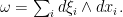
The cotangent bundle can be equipped by the canonical symplectic form 


where 


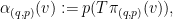
Now we define the following vector field 

One thing that might surprise you is that geodesics on configuration space
